19th Application of Computers and Operations Research in the Mineral Industry, R.V. Ramani, Editor. Sponsored by The Pennsylvania University, April 14-16,1986
Published by Society of Mining Engineers, Inc, Littleton Colorado 1986
Chapter 20, Pages 211-220
The Art of Cross Validation in Geostatistical Applications
Isobel Clark
Geostokos Ltd., 8a Lower Grosvenor Place, London SW1W OEN, England.
Abstract
Geostatistical methods of estimating ore reserves and other spatial phenomena are becoming increasingly wide spread in their use. Properly applied, Geostatistical estimation falls into two stages -- the "modelling" of the spatial variability within the study area; and the use of this spatial model to provide an appropriate estimation technique. The first stage usually consists of construction and interpretation of semi-variogram graphs, and the second is the development of the corresponding Kriging method.
Because of the apparent subjectivity inherent to the first stage of a geostatistical analysis, attempts have been made to provide methods of "testing" whether a particular semi-variogram model (say) adequately represents the study area. Increasingly, the choice of model is being justified by a process known as "Cross Validation". With this approach, the analyst uses a partial data set to estimate values at actual sampled positions. "Real" and "estimated" values are then compared in such a way that the model can be accepted or rejected.
This paper discusses the process of cross validation in some detail, using case studies as examples. Some problems with the technique are illustrated and discussed.
Cross Validation
The term "Cross Validation" seems to have been introduced into Geostatistical applications around the late 1970's. although the concept of comparing actual values with estimates is far older (cf. Krige 1959). David's Geostatistical Ore Reserve Estimation (1977 p.56) gives a fully worked example of comparing estimates from two different estimation methods with the "true" values from sampled areas. The purpose in this example is to show that the Kriging estimator gives a smaller error variance than an Inverse Distance Squared method. He suggests comparing the histograms of the two sets of errors, in addition to their respective means and standard deviations.
By 1979, Parker et al are using the term "cross-validation" to check that their method of prediction was the correct one. In that case, the variable of interest was the proportion of mineralised composites in a uranium deposit. In the same volume: Davis & Borgman mention "crossvalidation" as a procedure available to check the validity of a semi-variogram model; Rendu uses comparison of theoretical and observed means and errors to decide between kriging methods as does Clark. In three out of four studies, therefore, the purpose of the cross validation was to justify the kriging technique chosen to perform the eventual evaluation.
This method of cross-checking a technique seems to have been welcomed by workers seeking a method of reducing the amount of subjectivity in Geostatistical estimation. By 1983, the NATO ASI on Geostatistics contained almost a dozen papers which referred to cross validation as a method of testing the fit of the semi-variogram model to the data. The interest in the problem is reflected, also, by the number of papers on "robust" estimators and statistical fitting procedures. However, these are outside the scope of the present paper.
Historically, then, Cross Validation has grown from a virtually unknown technique in the mid-1970's to a routine tool in the Geostatistician's armoury. In addition to published papers, it is now common practice amongst consultants to include a chapter in their reports justifying the choice of semi-variogram model and (sometimes) the kriging technique selected for estimation purposes.
What is Cross Validation?
The term "cross validation" is now generally accepted as describing the following procedure:
- One sample is eliminated from the data set.
- The surrounding samples are used to produce an estimate of the value at this (now) "unsampled" location, using a Geostatistical estimation method.
- The actual error incurred in this process is measured by:
(Actual Value - Estimated Value)
- The "expected" or "theoretical" error is measured by the kriging variance calculated during the estimation process (or by its square root, the kriging standard error).
The procedure produces a list of actual and theoretical errors. At this point, however, authors diverge on what should actually be done with this list.
The most common procedure, judging by the literature, is as follows. The actual errors are averaged. If the estimation is unbiassed this average should be zero. The variance of the errors is calculated and compared with the average kriging variance for all the estimations. The ratio between these two quantities is expected to be one, if the estimation procedure has been carried out correctly.
A minor variation on this process was used by Clark (op cit) to take account of different standard errors where data are not taken on a regular grid. Each "actual error" is divided by the appropriate "theoretical standard error" to form a standardised (Z) statistic. These statistics should then average zero and have a standard deviation of one.
In all cases. then, the actual error is compared with the expected error in such a way that two statistics are produced. These are expected to be zero and one respectively. Achieving (0.0,1.0) becomes the "proof" that the original semi-variogram model "fits" the data. The logic which produces this conclusion is:
The correct model gives (0,1)
I get (0,1),
therefore the model is correct
It is with this logic that this paper concerns itself.
A Test Case
To illustrate the use of cross validation a set of data was simulated under ideal conditions for analysis by Geostatistics. To avoid distractions and concentrate on the investigation of cross validation, the deposit follows a Normal distribution, a specified semi-variogram model and has been densely sampled on a regular grid.
The simulation used for this case study is loosely based on a taconite deposit. The variable being studied is Iron and averages around 70%Fe by weight. The area is rectangular, 450 metres east/west and 300 metres north/south. It has been sampled, for the purposes of our study, on a 10 metre grid starting 5 metres in from the edge of the area. This gives 1,350 samples for the investigation.
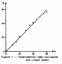
A semi-variogram was constructed for this data and is shown in Figure 1. A simple Linear model has been fitted to the graph by eye, and is found to have a slope of 1.00. There is no apparent nugget effect. The cross validation procedure was applied to this data set resulting in a set of "Z" statistics which had an average of 0.006 and a standard deviation of 0.907. The constant standard error, i.e. for points other than those around the edge, was 2.777%Fe.
Here we run into our first practical snag. We expect statistics of 0.0 and 1.0 if we have the correct model (and procedure). What significance is there in the fact that we have 0.907 instead of 1.000? It is quite remarkable that all case studies using cross validation in the literature quote figures which are very close to the ideal. There are no instructions as to how to interpret deviations from the expected statistics. Let us consider this particular case in detail.
A value of 0.907 for the standard deviation suggests that our "actual" errors are only 90% as large as the "theoretical" errors. That is, our semi-variogram model is being too pessimistic. Should we revise our model to achieve the desired statistic? This can be arranged quite simply because the kriging variance is directly proportional to the slope of the semi-variogram. If we adjust the slope of the model semi-variogram by a factor of 0.907*0.907 the error variances will become exactly equal, i.e. our Z standard deviation will be equal to 1.000. The constant kriging standard errors will become 2.519%Fe instead of 2.777%Fe. The estimates, however, will remain completely unchanged since these are independent of the slope of the model. (A similar effect would be achieved in the case of a Spherical model by scaling the sill value).
For this data, then, we would get Z statistics which averaged 0.007 with a standard deviation of 1.000 if we used a Linear semi-variogram model with slope 0.823. The only problem is that this line goes nowhere near the points on our experimental semi-variogram.
A Biassed Estimate?
Perhaps it would be a good idea to pause here to consider this problem. We expect a standard deviation for the standardised errors of 1.0. In the calculation above, we have calculated the standard deviation in the traditional way -- that is, the mean square deviation from the mean gives us the variance and we square root this to obtain the standard deviation. It is usual to divide the sum of squares by "n-l" to calculate the variance. The justification for this is that there are "n-l" independent pieces of information from which to calculate the statistic. In our case, this is patently untrue. Our sample values are highly related to one another and so are the estimates which we make of them. The errors for adjacent samples will also be related, although possibly not in such a simple fashion. Therefore, when we calculate a classical standard deviation -- whose derivation is based on independent samples -- we produce a biassed estimate of the real standard deviation of the Z statistics. Perhaps that is our problem here.
Figure 2 shows the histogram of the "Z" statistics. Theoretically, if we have the correct model this distribution should be Normal with mean zero and standard deviation one. Fitting a distribution to this histogram produces a mean of 0.006 and a standard deviation of 0.907. A χ2 goodness of fit test yields a statistic of 14.8 with 18 degrees of freedom. However, once again we are violating the conditions needed for the classical statistical test. A χ2 test assumes that the observations are drawn randomly and independently from the distribution.
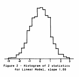
It would seem, then, that we need to find an empirical method of deciding whether our figure of 0.907 is significantly different from 1.000. If the deviation is due to our calculating classical statistics from highly unclassical data perhaps we can compensate for this by taking random subsets from the full data set.
Randomising the Statistics
In the discussion above, we used 1,350 inter-related sample values to estimate the standard deviation of the "Z" statistics. If our semi-variogram model is correct, we expect this standard deviation to be equal to 1.0. In an attempt to produce a more representative statistic, we will take a random subset of the samples and calculate the standard deviation from these. That is, we take our list of Z statistics and select (say) 150 samples at random from the list. We then calculate the mean and standard deviation of this smaller set of randomly drawn samples.
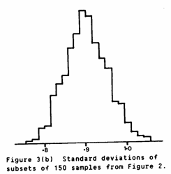
Rather than do this once and risk hitting an extreme value, the process was repeated 1,000 times and histograms constructed of the results. A subset size of 150 was chosen, Any other size could be chosen with little effect on the following results. Figure 3 shows the histograms of (a) the average Z statistic for the set of 150 samples and (b) the standard deviation of the sets of 150. Both of these histograms show no deviation from Normality. The average values of the subsets vary around the overall average, and range between -0.22 and +0.26. The standard deviations range from 0.74 to 1.05 and average 0.902.
It would seem that taking random samples from the complete set of cross validation statistics does not significantly change our troublesome value of 0.907. Rather, we must go back to the original data set, take our subsamples from that and perform the whole cross validation exercise with only (say) 150 samples. In this way, the estimates and standard errors are produced from a randomised sample. Thus, hopefully, the Z statistics should conform more to the requirements of our statistical approach.
Of course, we could take this procedure to its logical extreme and recalculate and remodel the semivariogram each time. This would be a pragmatic approach to a "jack-knife" technique. However, in the absence of an automatic method for fitting semivariograms, this is not considered practical.
Cross Validation of Subsets
A subset of 150 data points was selected from the original 1,350 sample values. A cross validation exercise was carried out on these 150 samples using a linear semi-variogram model with a slope of 1.00%Fe2/m and no nugget effect. The Z statistics were produced and their mean and standard deviation calculated. This process was repeated 100 times. A larger number would have been desirable, but the time factor proved prohibitive.
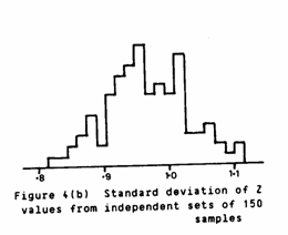
Figures 4(a) and (b) show the variation in mean and standard deviation of the Z statistics for these 100 subsets of 150 samples. These are directly comparable to Figures 3(a) and (b). Figure 3(a) shows averages of subsets of Z statistics from the cross validation on 1,350 samples. Figure 4(a) shows averages of Z statistics from cross validation of subsets of 150 samples from the original 1,350. That is, in Figure 4 only the 150 samples are used to produce the Z statistics.
Similarly Figures 3(b) and 4(b) show the standard deviations of the Z statistics in each case. Visual comparison of these graphs should be rewarding. It should be borne in mind, however, that Figure 3 is based on 1,000 subsets and Figure 4 on only 100. The lumpy nature of the histograms in Figure 4 is probably due to the small number of subsets. All four histograms give very good χ2 goodness of fit statistics when compared with a Normal distribution.
Comparison of Figures 3(a) and 4(a) show broadly similar shapes. The average in Figure 3(a) is 0.002, whilst that in Figure 4(a) is -0.011. The remarkable difference between the two is in the spread of values. The standard deviation in Fig.3(a) is 0.072 compared with 0.015 in Fig.4(a). That is, cross validations amongst a small set of data are far less variable than similar sized subsets amongst a large set. This is a little puzzling.
Comparison of Figures 3(b) and 4(b) on the other hand show similar "variation" amongst the standard deviations with 0.052 and 0.061 respectively. The major difference here is in the "central" average value. The small sets of data give a typical standard deviation of 0.967 whilst the subsets of the large set average around 0.902 (almost identical to the original 0.907). Combining this result with the one above leads us to the conclusion that the cross validation seems more stable on a smaller, scattered set of data than it does on a random selection from a dense regular grid. The small data subsets give final statistics of -0.011 and 0.967 to be compared against our "ideal" 0 and 1.
Conclusions from Cross Validation
From the limited study described above we can draw some tentative conclusions.
Although the technique leads us to look for statistics of zero and one there is no clear indication of how far our values can deviate from these "ideal" statistics. Since our samples are inter-related, classical statistical methods offer little help in either producing stable estimates of the statistics or in testing for significant deviation from the expected values of these statistics.
Two empirical methods of investigating the variability of the statistics have been used above. In the first, the list of 1,350 "Z" statistics has been subsampled many times over and the behaviour of these subsets examined. This produces well behaved graphs which vary around the average values produced by the whole data set. In the second, the original data set is subsampled and separate cross validation exercises are carried out on each subsample. This also produces well behaved graphs (allowing for the small number of subsets) but markedly different behaviour in the summary statistics.
It should be emphasised that this is a single example. There may be many cases in which the latter approach would give "worse" statistics than the former. What does appear clearly is that simply subsampling the Z statistics from the full cross validation exercise gives little extra information. Some computer packages give statistics on two "halves" of the data to illustrate how sensitive the cross validation is to removing some of the data. The end-user should ensure that these statistics are produced from two extra cross validation exercises and not just subsets of the original calculation.
Hypothesis Testing
Cross validation as described above is an example of what statisticians call "Hypothesis Testing". Most standard statistical tests are based on this procedure:
- A hypothesis is set up
- A "statistic" is derived (mathematically) that will have predictable behaviour if the hypothesis is true
- A value of the "statistic" is calculated from the data available
- This single value is compared to the distribution of expected values
In almost all cases the hypothesis set up is the opposite to that which is desired. For example, if we wish to deduce that two quantities are different we set up a hypothesis that they are the same. Then, if they are significantly different, the calculated statistic should deviate markedly from the expected behaviour. In other words, the value given by the data is a very unlikely one in the expected distribution. On this basis, the user will reject his hypothesis as unsatisfactory.
Notice, though, that this approach is hemmed about by circumlocutions. The final statement would be something like: "If the hypothesis is true, we have a 1% chance of obtaining a statistic as high as that given by this set of data". We have no right to say that, for instance, there is only a 1% chance that the hypothesis is true. We have even less right to say that there is a 99% chance that the hypothesis is untrue. In the final analysis a subjective decision must be taken. If a hypothesis is rejected at (say) the 1% level, we must accept the risk that the hypothesis is actually true and that we happen to have the one sample in a hundred which gives an extreme statistic.
On the other hand, suppose we obtain a value for the statistic which conforms to the "expected behaviour". Does this prove that the hypothesis is true? No, it does not. It tells us very little. It says: "there is no evidence from this calculation that the hypothesis is untrue". An "acceptable" statistic does not necessarily support the hypothesis but does lend it credence.
The Case Study Again
In the example detailed above, the (now) standard method of cross validation was illustrated on a large set of samples taken on a dense, regular grid. A semi-variogram was calculated and a model fitted to it. A hypothesis was set up that the model fitted the data. Z statistics were produced by Ordinary kriging. The expected behaviour of these statistics was that they would have a mean of zero and a standard deviation of one. After a little harmonising to reduce the non-independence aspect of the sampling, values of -0.011 and 0.967 were obtained.
These values would appear (intuitively) to be close enough to the expected values so that we may accept the hypothesis. We have no quantitative guide as to the risk factor involved here, except for the empirical information contained in the histograms in Figures 3 and 4.
This paper, so far, is a straightforward and (perhaps) unoriginal presentation of a technique now used routinely in Geostatistical applications. The remainder offers a rarer commodity -- the opportunity to investigate other models and compare their behaviour to the one detailed above. Because of the restriction on space, this study will consider only two other models and those only in brief.
Let us call the above model, i.e. Linear with slope 1.0 0 %Fe2/m, Model 1. At this point we will refer to the others simply as Models 2 and 3. In each case, the set of 1,350 samples has been used to produce a set of 1,350 Z statistics. In both cases the histogram of the Z's is acceptably Normal under the χ2 goodness of fit (hypothesis) test. Model 2 gives an average of 0.009 and a standard deviation of 0.921. Model 3 give -0.029 and 1.014 respectively. Under the cross validation approach, both of these models fit the data more closely than Model 1.
Choosing Between Models
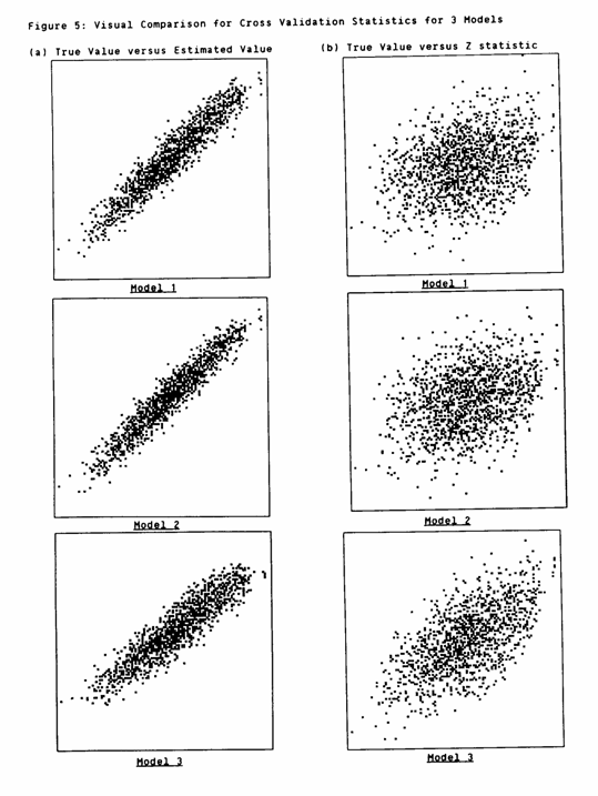
Three models have been fitted to the simulated taconite deposit and all of them produce acceptable cross validation statistics. We must look for some other way of comparing them before we can decide which is "best". Figure 5 illustrates a simple method of comparison, using scatter graphs of one quantity against another. Figure 5 shows (a) True Value (X axis) versus Estimated Value (Y axis) and (b) True value (X) versus Z statistic (Y) for each model. The value scale is 45%Fe to 92%Fe in each case and the scale for Z is -3.4 to 3.4.
In all cases the estimated values are highly correlated to the true values -- which is a desirable characteristic. In all cases the Z statistic is correlated with the true value, which is not so desirable. For Models 1 and 2 this correlation is around 0.34, whilst for Model 3 it is 0.64. Some correlation is expected between Z and the true value, because of the smoothing effect of kriging on point estimation. However, the high value given by Model 3 gives rise to some concern.
On the basis of Figure 5, then, there seems to be little to choose between Models I and 2. Model 3 seems to be a bit less desirable, giving too much smoothing on the estimates and marginally more scatter when comparing them with the true values.
Another method of comparison might be to try the "subsampling" approach used earlier to randomise the sample sets. This process changed the simple mean and standard deviation of 0.006 and 0.907 to derived parameters of -0.011 and 0.967 for Model 1. For Model 2 the new statistics are -0.003 and 0.978. Again we have no basis for choosing between 1 and 2. Model 3, on the other hand, gives new statistics of -0.60 for the mean and 1.547 for the standard deviation. At last we have a deviation from the ubiquitous zero and one. Although Model 3 cross validates nicely on the complete data set, on random sets of 150 samples it gives standard deviations between 1.3 and 1.8. These values would seem, intuitively, to be significantly different from 1.00. On this basis we could reject the hypothesis that Model 3 fits the data -- although we cannot quantify the risk factor involved in this decision.
The Models
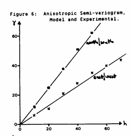
It is unusual, at least for this author, to judge the fit of a semivariogram without seeing experimental and model curves on the same graph. Figure 6 shows the experimental semi-variogram and Model 2 for visual comparison. It can be seen from Figure 6 that the deposit under study is, in fact, not isotropic. Only two directions are shown, these being the major axes of the anisotropy. The models for these directions are Linear with slopes 0.66%Fe2 /m and 1.25%Fe2/m. Intermediate directions have intermediate slopes varying in an ellipsoidal fashion. The cross validation procedure was unable to distinguish between an incorrectly fitted isotropic model and the "correct" anisotropic model.
Only the large number of samples enabled us to reject Model 3 as unsuitable, after the subsampling exercise. That model consisted of a pure nugget effect with the value 10.72%Fe2.
It should be fairly obvious that there are a large number of other models which are equally acceptable.
Summary
This paper has discussed the technique of cross validation, as currently practised, in more detail than hitherto. Two problems have been highlighted.
When a cross validation is performed how much deviation from the expected values of 0 and I can be accepted?
If acceptable values are obtained does this prove that the model correctly represents the data?
The conclusion which must be drawn from this study is that cross validation, as such, does not remove the subjective element from model fitting. However, it can be utilised as a data exploration tool via histograms, scattergrams and more detailed statistical exercises. The decision rests with the user with no clear assessment of the risks involved in an incorrect choice.
Many eminent authors have stated that the choice of semi-variogram model is virtually irrelevant since the final results - maps, block estimates, etc will be more or less the same in any case. It is a very simple job to demonstrate that this is untrue. But suppose it was true that the basic model is unimportant.
Then why are you using Geostatistics?
References
Clark I., (1979) "Does Geostatistics Work", Proc. 16th APCOM, pp.213.-225.
David M., (1977) Geostatistical Ore Reserve Estimation, Elsevier, 364p.
Davis B.M. & Borgman L.E. (1979) "A test of hypothesis concerning a proposed model for the underlying variogram", Proc, 16th APCOM. pp.163-181.
Krige, D.G. (1959) "A study of the relationship between development values and recovery grades on the South African goldfields", Journal of the South African Institution of Mining and Metallurgy, No.61, pp.317-331.
Parker H.M., Journal A.G., & Dixon W.C. (1979) "The use of the conditional lognormal probability distribution for the estimation of open-pit ore reserves in stratabound uranium deposits - A case study", Proc, 16th APCOM, pp.133-148.
Rendu J-M.M. (1979) "Kriging, logarithmic kriging, and conditional expectation: comparison of theory with actual results", Proc, 16th APCOM, pp.199-212.
Verly et al, (1983) Geostatistics for Natural Resources Characterisation (Proc. NATO ASI). D.Reidel, 1092p.