A case study in the application of geostatistics to lognormal and quasi-lognormal problems

Isobel Clark

Geostokos Limited, Scotland

ABSTRACT

The application of geostatistics to highly skewed data has always been problematic. Studies can be done using generalised “anamorphoses” or transformations, but these have limitations in mining applications. In particular, estimation and confidence levels on block and stope values can rarely obtained using these methods.

This paper considers the particular case of lognormal data and discusses the following:

Lognormal kriging and backtransforms;

Conservation of lognormality between point and block/stope averages;

The three parameter lognormal;

Distributions which are not exactly lognormal and associated problems.

These discussions will be illustrated with real case studies taken from mining applications from around the world.

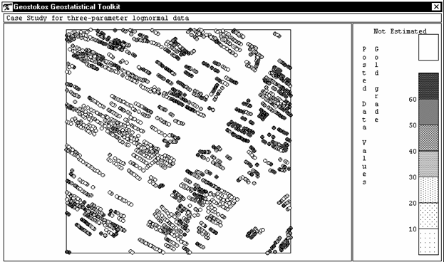Figure 1: sample data in 500m block within mine area

LOGNORMAL KRIGING

It is common knowledge that ordinary geostatistical methods do not deal well with highly skewed sample data. In recent times “distribution free” methods have been advocated to avoid this problem --- the most popular in practice, at this time, being the multi-indicator methods. As with all techniques, these have their strengths and weaknesses. One of the most obvious of the drawbacks to a multi-indicator approach is the necessity to model many semi-variogram graphs and to carry out many simultaneous kriging or co-kriging estimations. Where the distribution of sample values is reasonably simple and stable, it would seem more practical to use the known features of the distribution and associated methodology.

In this presentation we consider the simplest non-Normal case --- that of lognormal kriging. If the values within a deposit are known to be stationary and lognormal, then the logarithms of these values should be Normal. If all geostatistical analysis is carried out on the logarithms, there should be no problems with semi-variogram interpretation and modelling, or with kriging (whether simple or ordinary). Universal kriging may also be used if the residuals from the trend in the logarithms of the sample values can be assumed to be Normal. The only potential problem is in the “backtransformation” of the logarithmic estimates to the original sample value scale. There appears to be some disagreement in the general geostatistical literature as to how this backtransform should be carried out.

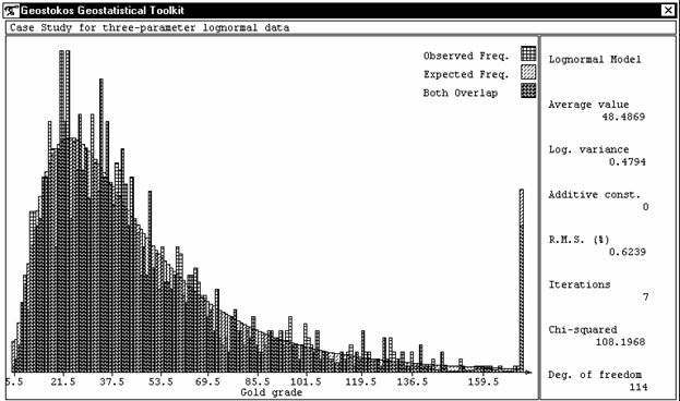Figure 2: histogram of sample values and fitted lognormal model

We illustrate this paper with a case study on a Witwatersrand type reef. Figure 1 shows the layout of sample values taken within an area 500m by 500m of the reef. The values measured on these samples can be shown to have a lognormal distribution (Figure 2). Logarithms of the data values were taken; semi-variograms calculated and fitted; and a cross validation exercise was carried out. The kriging produces an estimator for the logarithm at each location and a kriging standard error (square root of the kriging variance) associated with that estimate. There is little problem applying the standard geostatistical analysis to this well behaved Normal data set.

This case study is based on a simulation of ideally lognormal data to ensure that complications are avoided. Later in the paper we discuss some real cases where a lognormal approach does or does not produce acceptable results. Because this is a simulation, we know the actual values for a 1 metre grid over the area. Panels of various size – from 5 to 100 metres – were kriged and compared to the actual values from the simulation.

Figure 3: comparison of various backtransformations

To obtain values in the original units, it is necessary to carry out a backtransformation. Unfortunately, simply anti-logging the values does not produce unbiassed estimators. In Figure 3, we have plotted the results for 50 metre panels (purely for clarity). We can see that the anti-log does not match the “actual” panel value very well at all. The correct backtransformation for the lognormal case contains the following terms:

· The kriging estimate for the average logarithm;

· One-half of the kriging variance for this estimate;

· One-half of the “within panel” variance term (used in calculating the kriging variance);

· The lagrangian multiplier from the solution of the kriging equations.

The backtransform is found by subtracting the last term from the sum of the first three and then taking the anti-logarithm. This can also be expressed as a function of the “between panel variance” and the “between estimate variance”. Computationally, the expression above is simpler, since all of the terms are used in or produced by the kriging system. Some practitioners in this field have suggested that the last term is superfluous in practice, since it generally averages out to zero. For this example, the lagrangian multipliers average 0.2021, resulting in a factor of around 81% on the final results. Figure 3 shows the estimators before and after the application of the lagrangian multiplier, clearly illustrating the importance of this factor.

The complexity of this backtransform suggests that a general “anamorphosis” will be rather more complicated than a simple forward and backward transformation. One popular misconception is that the major difference between the “correct” backtransform and a simple anti-log (say) is due to the difference between the variance of panel values and the variance of the kriging estimates. It can be seen in Figure 4 that the standard deviation of the kriging estimates is somewhat lower than the standard deviation of the logarithm of the actual panel values.

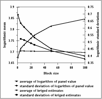
Figure 4: relationship between logarithmic parameters for backtransforms

However, it can also be seen from Figure 4 that there is a significant difference between the average of the logarithm of the actual panel values and the average of the (untransformed) kriged values. For example, for the 50 metre panels, the standard deviations differ by 0.05 whilst the averages differ by almost 0.2. The full backtransformation includes a correction factor for the difference in the logarithmic means in addition to the generally accepted correction on variance.

The conclusion which must be drawn from this is that backtransformation is not just a question of variance correction. Cognisance must be taken of the shape of the distribution as well as the spread of values. The Normal distribution retains the same shape no matter what variance the values take. No other distribution has this property. In this simplest of cases, where the values are Normal when logarithms are taken, all of the parameters of the distribution change with panel size and with weighted average estimation techniques. To obtain unbiassed estimates for the original data units, both mean and standard deviation of the logarithms must change. Extreme caution must be observed in using transformations which only rely on variance corrections and constant distribution shape.

One point which cannot be emphasised too strongly is the importance of the correct semi-variogram model. In particular, the absolute sill value – which is of relative unimportance in Normal applications – is crucial in obtaining realistic backtransformations. This is one case where the cross validation technique can prove extremely useful. The cross validation exercise should be set up so that it also checks on comparison between the actual (untransformed) sample values and the backtransform of the estimates. If the average “actual” value is close to the average backtransform, we can have more confidence that the backtransform will work with unsampled locations.

CONSERVATION OF LOGNORMALITY

Another question which arises when applying lognormal kriging is the so-called “conservation of lognormality”. The validity of the backtransform relies on the panel (or block) averages retaining a lognormal distribution. There is absolutely no theoretical reason why this should be so. However, it appears to be the case in many practical applications. In this simulated case study, no matter what block size is taken the resulting values are lognormal.

Perhaps this would form a good diagnostic of the likely stability of a lognormal estimation method. If a densely sampled area (or volume) is available, panel (or block) averages should be calculated and their distribution investigated. This could also form the basis of a useful “declusterising” technique.

PRACTICAL CASE STUDIES

It is not possible to give complete case studies in a paper, but we will discuss some practical applications here briefly.

A. Platinum, USA

Sample values in a certain platinum mine follow a moderately skewed distribution. Figure 5 shows a histogram of the sample values with a fitted lognormal distribution. It is fairly obvious that the data does not follow the ideal behaviour which would allow us to use lognormal kriging.

However, with the introduction of an “additive constant” this data becomes acceptably lognormal. With this model, we simply add a constant value to each sample value before taking logarithms. This model was first suggested by Sichel in the 1950’s when the ideal lognormal was found inappropriate in many South African applications. Figure 6 shows the same histogram with a three parameter lognormal model fitted.

Lognormal kriging can be applied with confidence to the three parameter lognormal. Since the additive constant is added before the logarithmic transformation, it must simply be subtracted from the final answers after backtransformation.

Figure 5: histogram of sample values with fitted lognormal distribution

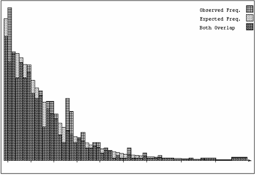
Figure 6: histogram of sample values with fitted three parameter lognormal distribution

B. Zinc, Namibia

A recent project in Namibia involved estimation of blocks for planning an open pit. Borehole cores had been coded for host rock type and the data set split accordingly. The majority of the mineral was hosted in a single rock type. When the histogram of values was plotted, the values were seen to be highly skewed (Figure 7). This is fairly unusual for a base metal deposit. However, a logarithmic transform does not normalise this data. Instead, it produces a histogram which is apparently negatively skewed (Figure 9).

The reason for this strange behaviour becomes clear when the values are plotted using probability scales (Figure 8). On “probability paper”, a Normal distribution shows as a straight line. From Figure 8, we can see that a large proportion of the samples appear to belong to a Normal distribution. However, the lower tail of the distribution seems to comprise a separate positively skewed component terminating at zero. In the upper values, the expected proportion of very high values is not realised in the samples available.

On closer investigation, it was found that there were three phases of mineralisation within this single host rock plus an oxidation zone in the 10-20 metres below the surface. This is an ideal case for multiple indicator kriging, perhaps linked with ordinary kriging within broad grade divisions.

Figure 7: Zinc values, Namibia

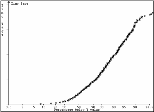
Figure 8: Zinc values, Namibia

Figure 9: Zinc values, Namibia – logarithms

C. Gold, Zimbabwe

For our third example, we consider a greenstone type gold deposit in Zimbabwe. The probability plot of the logarithm of the sample values is shown in Figure 10. According to this graph, the values are not lognormally distributed, since there is a significant and consistent deviation from the straight line at the lower end of the plot.

These samples are taken from the stoping areas in an underground operation. The apparent anomalies in the distribution are common in producing mines. This is because the areas mined tend to be those which are economically profitable. In simple terms, mining does not normally take place in poor and uneconomic areas. Therefore, when we look at the sample histogram or probability plot, we have (effectively) a filtering of the lower values due to lower coverage of the poor areas.

Because “unpay” ground tends to be intermingled with “pay” ground, there will be lower values in the most profitable of stopes. There will also be higher values left unmined in generally poor areas. The impact on the probability plot is that seen in Figure 10. The “wave” at the lower end of the graph reflects the omission of some of the lower values. The drop-off at the upper end of the graph reflects higher values missed because they are included in blocks of ground which are, on average, uneconomic. Although new models have been evolved to deal with this type of distribution, the shape of the graph is, in effect, an artifact of the way the samples are collected and does not reflect the true population behaviour for the whole deposit.

In this case, it was verified that simple lognormal methods were acceptable for grade control and production mine planning.

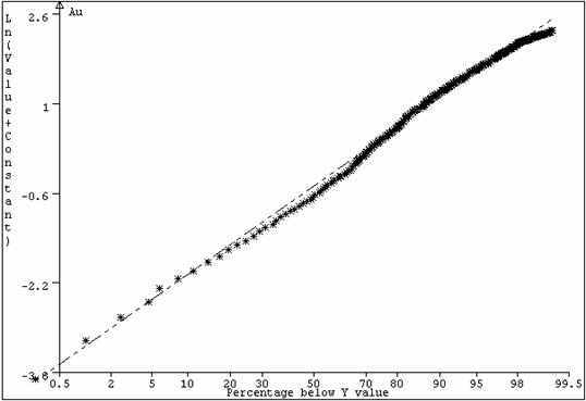
Figure 10: Gold values, Zimbabwe