J. S. Afr. Inst. Min. Metall, vol. 87, no. 10. Oct. 1987. pp.293-306.
Turning the tables – an interactive approach to the traditional estimation of reserves
by ISOBEL CLARK*
*Managing Director, Geostokos Limited, 36 Baker Street, London WIM IDG, U.K.
© The South African Institute of Mining and Metallurgy, 1987. Paper received 24th January, 1986. SA ISSN 0038-223X/$3.00 + 0.00
SYNOPSIS
This paper reviews some of the traditional methods of reserves estimation based on lognormal distribution with or without an additive constant. In the rush to computerize mine planning and grade control generally, proven estimation methods, such as Sichel's t, seem to have been overlooked.
By use of a personal microcomputer, the traditional methods were investigated thoroughly, the results being tested against existing tables and figures.
The fitting of a lognormal distribution, including estimation of the additive constant, is discussed, and the calculation of Sichel's t estimator and its associated confidence limits is described in detail. Payability calculations for a lognormal distribution are also covered briefly.
The advantages of personal computers, particularly speed and ease of use, are emphasized. This low-cost approach permits detailed investigation of some of the assumptions and approximations inherent in the established methods of calculation. Several disturbing discrepancies are revealed in various factors, and some generalized statements made by previous authors are found to be over-simplistic.
Full details are given of acceptable approximations and computer algorithms, and concern is expressed over the possible loss of proven methods under the welter of new, sophisticated computer software.
Introduction
The development and availability of personal computer power over the past few years have been phenomenal. The proliferation of manufacturers, operating systems, suppliers, and packages leaves the potential user breathless and (sometimes) bewildered. Whatever the choice of hardware the trend worldwide seems to be away from the giant mainframe computer towards the minicomputer and microcomputer.
In this day of the 'personal computer on every desk', perhaps it is time to re-appraise some of the techniques that are traditionally carried out with pencil, calculator, and definitive tables. These methods, which have proved their value over any years of operation, can be emulated on computers of any size. Why, one asks, has this not been done?
The main resistance to computerization seems to have been twofold. The inaccessibility and sheer cost of calculating (say) a Sichel's t estimator on a mainframe has been a major discouraging factor. Secondly, the need to acquire considerable computer expertise before being able to operate such systems persuaded all but a dedicated few to stay with the tried and trusted calculation methods. The advent of personal computers and the benefits of 'user friendly' software have removed both of these problems.
This paper discusses three of the typical tasks undertaken at various stages of reserve estimation:
((a) the determination of lognormality of sample values and the possible choice of an 'additive constant' for the three-parameter lognormal;
((b) the calculation of Sichel's t estimator and associated confidence levels for two- or three-parameter lognormals; and
(c) the calculation of pay limit/pay value/percentage payability, which is generally undertaken with the use of such graphs as Krige's GRL20.
The purpose of this paper is simply to discuss the implementation of the traditional practices on a digital computer, as has been done at Geostokos, London. Some advances in numerical techniques will be presented, but in all cases the underlying theory remains the same as that which has been proved in practice over the past forty years.
The Lognormal Distribution
All the tasks described above relate to the application of the lognormal distribution to sampling and estimation problems. Traditionally, samples are assumed to come from a lognormal type of distribution, sometimes modified by the introduction of a third parameter – the 'additive constant'. The efficacy of this approach in practice has been proved time and time again, particularly in its application to the problems of the Witwatersrand gold reefs. Other minerals too uranium, for example – have been found to follow the three-parameter lognormal. This has enabled workers to produce more reliable estimates for grades and tonnages in these situations.
A typical approach to an estimation problem, then, would be to estimate values for the parameters associated with the relevant lognormal distribution and then to use these values to carry out payability calculations for the study area. The values that need to be estimated are the additive constant (if any), the average value, and the logarithmic variance of the distribution. Several methods are available for this calculation, but this paper confines itself to the traditional approaches that use logarithmic probability plots and the t estimator developed by Sichel.
The Fitting of a Lognormal Distribution
In the late 1940s, the first 'probability' paper became available. This graph paper is used for the plotting of data value (generally on the vertical axis) versus the percentage of samples below the data value (horizontal axis). In the standard probability paper, the 'value' axis is arithmetic. The percentage axis is constructed in such a way that a set of samples from a normal (Gaussian) distribution produces a straight line. The data value corresponding to the 50 per cent point is taken as an estimate of the mean of the distribution. The standard deviation can be calculated directly from the slope of the line – the usual procedure is to take the difference in value for the 84 and 16 per cent points and divide this by 2.
There is no clear indication of the first use of probability paper in the mining industry, but this must have followed closely on the heels of its invention, since it was in common usage by the 1950s. For the lognormal distribution, the arithmetic value scale is replaced by a logarithmic scale. In this way, a set of samples from a lognormal distribution will give a straight-line fit. The 50 per cent point is now the median, and the logarithmic variance can be determined from the slope of the line, as before.
In general, the procedure would be something like this:
(1) construct a histogram from the sample data;
(2) calculate 'cumulative' frequencies, i.e. number of samples below a given data value;
(3) calculate the percentage of samples below a given value;
(4) plot 'data value' on the logarithmic scale and 'percentage of samples' on the probability scale; and
(5) by eye, fit a straight line through the points.
The judgement of whether the line 'fits' the points is a subjective one. However, experience has shown that there is seldom any ambiguity about the decision – it either fits or it does not. The process can be refined by the application of a statistical test, such as the ᵡ2, to check the fit of the samples to the distribution.
The Third Parameter
Once probability plots came into common use, it soon became apparent that the lognormal distribution did not always fit the sample data. A common occurrence was a sharp downturn in the data at the lower end of the graph, giving significant deviation from the straight line. In 1960, Krige introduced a third parameter – the additive constant – into the analysis. Instead of the sample value being plotted on the logarithmic scale, the value plotted was 'sample value + constant'. This has the effect of raising the downturn so that the line straightens out. The criterion for the 'best' value for the additive constant is that in which 'the plot of the points best resembles a straight line' (Krige, p. 7). The process of estimating the third parameter is not a simple one. The additive constant must be included in the data value before it is plotted on the logarithmic scale. This changes every point in the graph – not just those off the line. Strictly, then, one should plot a graph for each possible value of the additive constant and then select that which gives the straightest' line.
Rendu (p. 7) suggests an arithmetic means of arriving at the additive constant based on the 50 per cent point and two complementary percentile points. Current usage favours the 16 and 84 per cent points for this calculation. This drastically reduces the amount of calculation and plotting involved. However, Rendu notes that 'It is therefore important to check graphically that the cumulative distribution of x+β is lognormal' (where x is original sample value and β the constant). In other words, one still has to decide whether the line is straight when the third parameter is included in the analysis. If Rendu's formula 2.13 does not give a straight line, one must revert to trial-and-error methods or reject the three-parameter approach.
The Digital Computer
This process seems to be an ideal candidate for the special abilities of a digital computer. The criterion for the 'best' fit has been clearly stated as the straightest fine. The actual computation procedure is simple enough, but is extremely tedious. The computer is the ideal tool to carry out this type of repetitive calculation swiftly and without error.
The process can be summarized simply as follows:
(a) choose an additive constant,
(b) construct a probability plot,
(c) fit a straight line through it, and
(d) measure deviations from the line.
This procedure can be repeated for many values of the additive constant in a fraction of the time it would take to tackle one value manually. The only numerical complication is in the construction of the 'probability' axis. Many algorithms are available for this. This author favours the use of JRSS Algorithm 111 by Beasley and Springer, which is a FORTRAN subroutine called PPND – 'Percentage Points of the Normal Distribution'. This routine provides the standard normal deviate associated with any given percentage of samples.
There are, of course, many methods of fitting a straight line through a set of points. At Geostokos, we favour the standard least-squares approach, choosing to minimize the difference between the 'percentage of samples' and the 'percentage of lognormal distribution' below a given data value. In fact, this measure can be used at both stages:
once an additive constant has been chosen, the best line minimizes the difference between observed percentage and expected percentage;
for a set of additive constants, the best line is the one with the smallest minimum difference.
In plainer language, the set of parameters that 'best resembles a straight line' is the set that produces the smallest differences between the observed percentage and the expected percentage as measured by the sum of squares of these differences.
A Computer Program
In our computer implementation of this method, we work on the assumption that the data really do come from a three-parameter lognormal distribution. This may sound trite, but few computer programs are written to argue with a user who is determined to apply an inappropriate analysis.
The practical consequence of this assumption is that, if successive values are taken for the additive constant, the line will gradually straighten out until the correct value is reached and then start to curve again in the 'Opposite' direction; that is, there is a best-fit line somewhere. In practice, we have programmed our software to stop if the additive constant becomes larger than the largest sample value and a minimum has not been reached. This is an arbitrary (but sensible) stopping rule.
Our program chooses a starting value for the additive constant, and successively raises this by increments until a minimum has been found and passed. To save unnecessary computation, a fairly large increment is chosen. This increment is then reduced, and the region around the supposed minimum is searched for a more precisely defined minimum. This process can be repeated until the required precision is reached. We have found that a starting increment equal to around one-tenth of the first histogram interval gives a satisfactory compromise between speed of operation and the number of repetitions required.
Timings for this sort of procedure vary considerably. A histogram with a large number of intervals and a high value additive constant will take the longest run time. The example given as Figure 5 by Krige (p. 7) takes less than 10 seconds on a standard IBM PC without coprocessor. An example with 120 intervals and an additive constant half way through the range may take up to 2 or 3 minutes.
Perhaps it is worth noting that, if one does not have enough samples to build a histogram, the above process works equally well on ungrouped sample data.
A Statistical Approach
The technique described above is the traditional approach and merely emulates on a computer what analysts would normally do by hand. The computer chooses successive additive constants and checks which one gives a set of points that most resembles a straight line.
However, there are many other ways of trying to solve the same problem. For example, in the late 1960s Sichel's studied (at some length) generalized moment methods for moderate to large sets of samples. He pointed out that, for small sample sets from this sort of distribution, ordinary moment methods can be distinctly unstable.
One statistical approach to the problem of fitting a three-parameter lognormal distribution to a set of sample data is briefly discussed here. Using exactly the same approach as the traditional one, the aim is to minimize the difference between the observed percentage of samples below a given value and that predicted by a distribution model. In fact, as described above, the sum of the squared differences is minimized.
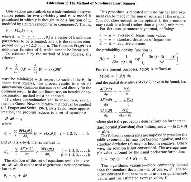
Now, one has a set of observed percentages and can specify the distribution model by giving values to the three parameters - mean, variance, and additive constant. This is the classic least-squares problem. The only difficulty is that the classic least-squares approach does not give a set of linear equations that can be solved for the 'best' values of the three parameters. Instead, it gives a set of equations that are non-linear. The non-linear least squares (NLLS) problem has been discussed fully elsewhere"," and is very simple to implement on a computer. The application of the NLLS approach to the three-parameter lognormal fitting is described in Addendum 1.
There are two practical implications in the application of the NLLS method. Firstly, this kind of 'iterative' method requires a 'starting point' – that is, one has to provide first guesses at the values of the parameters. Secondly, it can be seen in practice and proved in theory (MacDonald, personal communication) that the NLLS method tends to be less influenced by erratic values in the tail of the distribution and more by the whole shape of the curve. This is a distinct contrast to either moment methods or probability plotting. We have found a happy compromise in the use of probability plots to provide the initial estimates for the NLLS routine.
The Additive Constant
Krige has noted that the choice of additive constant seems to have little effect on the final estimate of the average value. This is true when the average value is estimated directly from the probability plot or when NLLS is used. However, the logarithmic variance can be unduly influenced by a change in additive constant – by up to 50 per cent in some cases. In addition, if the constant chosen is used in a Sichel's t type of estimation, the average grade may also be affected, since the optimal estimator depends heavily on the logarithmic variance of the samples.
Table I shows a set of 15 (simulated) samples from a three-parameter lognormal distribution with an additive constant of 100. Table II shows the effect of feeding different additive constant values into a Sichel's t computation. One interesting feature of the results is that the logarithmic variance declines steadily as the additive constant rises. The other point of interest is that, despite this feature, the estimated mean value stabilizes once the 'true' value of the additive constant has been reached. Have we, perhaps, struck another empirical tool in deciding the value of the additive constant?
In
short, then, the choice of additive constant for small sets of samples could be
crucial if a more 'objective' estimator of the average grade - say, Sichel's t
- is to be used and if confidence levels are to be calculated.
Although the estimator and (strangely enough)
the lower confidence levels stabilize fairly quickly, the logarithmic variance
and the
Thus, the extra effort of obtaining 'good' estimates of the logarithmic variance will be repaid in more accurate confidence levels and pay limit calculations.
Estimation of Maximum Likelihood
The previous discussion covered two approaches to the fitting of a lognormal distribution to a set of sample data. The use of probability paper to fit a straight line - either empirically or by Rendu's shortcut – is essentially an intuitive least-squares approach. The other method put forward for consideration was an iterative NLLS approach, requiring initial estimates for the parameters involved in the lognormal model.
Almost forty years ago, Sichel, first put forward his method for the estimation of maximum likelihood for the average value of a lognormal distribution and for confidence limits associated with this estimator.
The criterion of maximum likelihood is (in simple terms) a method of finding the model distribution from which samples are 'most likely' to have come. It can never be emphasized too much that measures of probability (like least squares) calculate the likelihood of samples coming from a given model population. They do not calculate the probability that the model fits the data but rather that the data fit the model. This is not at all the same thing, especially when it comes to the evaluation of such concepts as confidence intervals.
Sichel, then, evolved the theoretical background to an estimator of the average of the lognormal distribution and associated confidence levels on this estimator. This theory has been substantiated by almost forty years of practical use, the major developments over the years being updated and more accurate tables for the various factors. The production of Sichel's tables, specifically those given in the 1966 paper was programmed expertly by Vera Marting. However, no details on the computer algorithms or approximation techniques are given in the paper.
The tables currently in use are those published by Wainstein in 1975, which have been copied and quoted in many other papers and textbooks (e.g. Rendu, David). Although Wainstein extensively described his computerization of the Sichel t approach, his quoted computer costs and timings were prohibitive and seem to have discouraged other workers from tackling the same problem. With timings such as 61 minutes to produce a single A(T) integration on an IBM mainframe, Wainstein needed to use approximation techniques to obtain his final tables for the Ψ factors. The computerization that is fully described here is a workable compromise between mathematical exactitude and response time on a microcomputer. The results can be shown to achieve an accuracy of 99,998 per cent for all the factors, provided that there are at least five samples in the data set. For four samples, the accuracy achieved was only 99,98 per cent.
Sichel's t Estimator
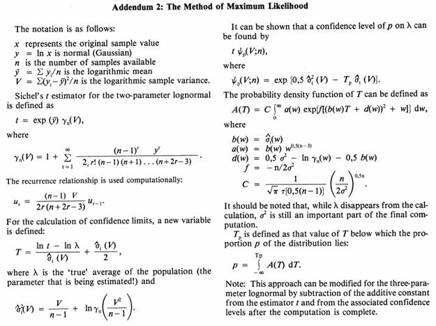
The mathematics of Sichel's maximum likelihood estimator are extensively documented in Sichel's own papers and by Wainstein. For completeness, the bare bones of the mathematics are given in Addendum 2. In this part of the paper, the discussion is couched in intuitive terms and slanted towards the implementation of this established estimation method on microcomputers.
Sichel's t estimator was developed for a two-parameter lognormal distribution. This is discussed in detail in this section of the paper, with an indication at the conclusion of how the estimates should be adjusted in the three parameter case. Sichel's notation is used throughout, except where this conflicts with the notation (Krige's) established earlier in the paper.
The first stage in this type of estimation is to take the logarithm of each sample value. For simplicity, the natural logarithm (loge or ln) is taken. The use of logarithms to the base 10 simply leads to the introduction of an unnecessary constant. The average of these logarithmic values is calculated (ybar), as is the sample variance (V). It is emphasized that V is the sample variance since it is the average squared, deviation from the sample mean. This is the maximum likelihood estimator for the logarithmic variance; it is, however, a biased estimator for the logarithmic variance. By tradition, then, V has always been used in Sichel estimation rather than the unbiased estimator (s2).
Development of the likelihood theory reveals that the 'best' estimator of the average value of the lognormal distribution is the anti-logarithm of the logarithmic average multiplied by a factor that depends on the number of samples (n) and the logarithmic sample variance (V). This factor is referred to as γn(V) in all the literature. The mathematical expression for γn(V) is a summation of an infinite series of terms involving n and V. This presents few computation difficulties except for the usual ones of rounding error and stopping rules.
The first problem concerns the number of terms actually to be summed, i.e. what is the approximation to infinity in this context? We use the simplistic approach. Once the next term to be added to the series becomes smaller than our 'precision' criterion, we stop. We have found that a figure of 0.000001 (10-6) is adequate to reproduce all the published figures. The use of smaller figures seems to have no effect on the calculations.
The second problem, especially with microcomputers, is the possible rounding error introduced by the calculation of the individual terms in the summation. Three figures are raised to powers, and two factorial type expressions must be evaluated. We have taken the simple precaution of using a recurrence relationship to calculate the next term in the series from the previous one. The expression is given in Addendum 2.
The execution time for the calculation of γn(V) is negligible, even on a microcomputer. We have not carried out any detailed timing runs for this factor.
Confidence Levels
The real computational difficulties are encountered in the evaluation of confidence levels for the Sichel's t estimator. Although the t estimator is the 'best' estimate for the true average value of the lognormal distribution, it is often vital to know just how accurate this estimator is. The traditional approach to this question has been the production of 'confidence levels'. These calculations give an idea of how 'close' the estimate could be to the true value. This permits the association of a measure of confidence to (say) the payability of an area to be mined.
The classical approach to the calculation of confidence levels is as follows:
(1) establish what estimator to use for the parameter,
(2) derive the probability distribution of that estimator,
(3) specify a level of risk that is acceptable,
(4) find the corresponding percentage point on the distribution of the estimator, and
(5) measure how far this is from the 'true' (expected) value of the parameter.
Sichel's papers detail the form of the estimator (described above) and derive the probability distribution theoretically. The problem is merely to program this on the computer. The mathematics is given in Addendum 2. The implementation is discussed here only in the simplest terms.
The estimator (t) is a statistic calculated from a given number of sample values ( n). Another set of n samples would give a different set of values, which would yield a different t value. A hundred such sample sets would yield a hundred potentially different t values. However, these t values would present some sort of predictable behaviour, because the distribution the samples come from is known and there are always the same number of samples. Mathematically, then, Sichel derived a formulation for the distribution that would be expected if lots of t statistics could be produced. In fact, the distribution he obtained was for a function of t that he denoted T (Addendum 2). Sichel calls this probability distribution of T values, A(T).
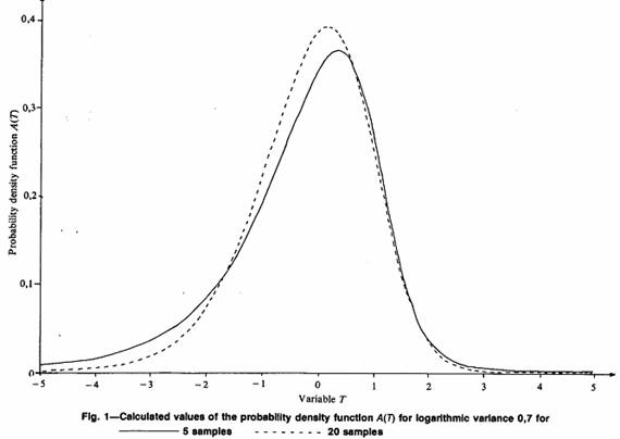
The probability density function (p.d.f.), A(T), shows the distribution of possible T values with respect to the 'true' average value of a lognormal distribution for a given number of samples. The p.d.f. A(T) depends on two major factors: n, the number of samples used in the estimation, and σ2, the logarithmic variance of the lognormal distribution; that is, a different n will give a different shape to A(T)(Fig. 1). So will a different σ2 (Fig. 2). Here is the first real problem in the calculation of confidence levels for a Sichel's t estimator. One generally knows how many sample values one has. However, very rarely does one know the true logarithmic variance of the whole distribution.
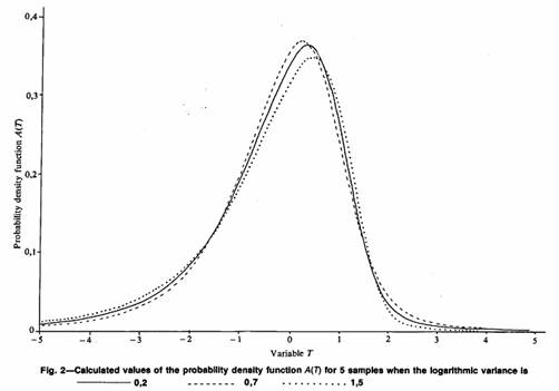
Both Sichel and Wainstein mention this problem. Sichel states that the A(T) distributions are virtually identical in the region 0.3 < σ2 < 1.5 and suggests that the selection of σ2 = 0.7 is an acceptable compromise. Wainstein produces a table comparing the percentage points actually obtained if σ2 is assumed to be 0.7 when it is not. He concludes that the decrease in accuracy is negligible within the above range. Wainstein makes no recommendations as to what action to take if (say) σ2 = 3.0. Some simple comparisons on the resulting Ψ factors for σ2 = 0.7, 0.3, σ2 = 1.5, and σ2 =n V/(n–1) are shown in Table III.
Table III lists a subset of the usual range of V values and a fixed number of samples (10), and illustrates the differences for the upper 95 per cent confidence level. It can easily be seen that the Ψ factors change with the assumed value for the 'true' logarithmic variance. A smaller true variance leads to a smaller Ψ value. This makes some sense since, if the original values are less variable, the estimates of the mean should also be less variable. A closer inspection of the values in Table III shows that, for small V (small observed variance), the differences between the columns are minor, amounting to 1 per cent at most. For 'usual' values of V, around 0.6, or 0.8, with σ2 = 0.3 instead of 0.7, the Ψ value is over 6 per cent lower; at σ2 = 1.5 there is a similar discrepancy. The use of the 'best unbiased estimator' of σ2 (s2) = n V/(n – 1)) obviously gives around the same value. For an observed sample variance of 1.5, the differences mount to between 12 and 13 per cent. At V= 2.0, there is a 12 per cent difference between σ2 = 0.7 and σ2 = 0.3.
For σ2 = 1.5, the, difference is 16.5 per cent, and for σ2 = s2, 28 per cent.
It would appear, then, that changes in the assumed value of the true logarithmic variance can affect the calculated Ψ factors by up to 30 per cent in situations that are hardly extreme. For the lower confidence levels, which are perhaps more important in practice, the discrepancies are not so high, although they are still significant. To assume a blanket value of 0.7 for the true variance when we provide tables for observed variances between 0.01 and 3 seems a little unrealistic. It is felt that this question of the assumed variance has been dismissed too lightly in the past and warrants further in-depth investigation. However, that is not within the scope of the present paper.
Calculation of A(T)
As stated above, the probability density function for T, A(T) , is a function of the number of samples used (n) and the true logarithmic variance (σ2). The value of A(T) for a specific value of T is an involved expression in T, n, and σ2, and is given in Addendum 2. In fact, it involves an integration of a complicated function over the range zero to infinity. The calculation of this function on a computer, then, depends on the numerical evaluation of this integral.
There are many methods of numerical integration sometimes known as quadrature (Abramowitz and Stegun). In all these methods, the formula is evaluated at intervals over the range of integration. These values of the function are combined in a weighted average, which approximates the integral. Intuitively, the smaller the interval, the more accurate the numerical approximation. However, the smaller the interval, the longer the calculation time. One must decide, then, what interval achieves the necessary precision on the integration without making the calculation time prohibitive.
In this particular integration, there is also the problem of when to stop integrating, i.e. what is the approximation to infinity. There are three decisions to be made, then:
(a) what method of numerical integration to use,
(b) what interval for discrete approximation to use, and
(c) what approximation to infinity is sufficient.
Although it would be possible to choose these factors based on strict mathematical criteria, we have chosen to do so empirically. We chose as our criterion those factors which produce a probability density function that is accurate to five figures (99,999 per cent). We feel that this is adequate for all normal usage.
Abramowitz and Stegun (Section 25.4) give around three dozen different methods of numerical integration and their associated precisions. We experimented with five of these and found little difference between the final accuracies achieved. Finally we settled for the extended Simpson's Rule, which satisfied our operating criterion.
The selection of an approximation interval is, of course, tied into the integration method chosen. We found that an interval of 0.010 was sufficient for n > 5. Some loss of precision was experienced for n = 4 (99,98 per cent) and more for n = 3 (99,64 per cent). However, we could not obtain any improvement on this by taking smaller intervals in the integration. This may be a reflection of the instability of the mathematics for n < 5, rather than computational problems! It was decided that an interval of 0.010 was adequate for normal usage, 0.005 being used for further investigative purposes.
Detailed investigation revealed that the number of intervals needed – or the range of integration – depends greatly on n. The higher the value of n, the lower the range of integration needed. We decided on a fixed range that would serve all n values. This means that more computation is carried out than is needed for large n values. However, we feel that the time saved by altering the range would be offset by testing for the range actually required. The final decision was to take the value 5.0 as our approximation to infinity. At an interval of 0.010, this means 500 intervals. For an interval size of 0.005, we need 1,000 intervals.
Our main timing runs were carried out on our in-house microcomputer, an Alpha Micro 1000 machine. This system is approximately four years old, and was one of the first systems based on the M68000 16-bit chip. We use a FORTRAN 77 (full) compiler. However, the approaches described can be implemented in any high-level scientific language. All timings are 'real time' not CP time – that is, the actual subjective time taken to run the calculations on a one-user machine.
Timings need to be split into two parts. There is an 'overhead' time in calculating the multiplicative factors at various intervals. This remains fairly constant at around 19 seconds for odd values of n, and 24 for even values. The difference is caused by the calculation of the T function in the overall constant (Addendum 2). Once the overhead calculations have been carried out, single values of A(T) can be calculated in under a second (for values in the tails), with some points taking upwards of 5 seconds (central values for n<10).
In summary, we evaluate the probability density function of T using the Extended Simpson's Rule numerical integration method. We integrate over a range 0 to 5 using an interval of 0.005 for our investigations. This gives better than 99,98 per cent for all n > 3. All of this evaluation was carried out with σ2 = 0.7.
Evaluation of Confidence Levels
We can now evaluate (and graph) the probability density function for the T statistic from a given number of samples. We can, therefore, investigate the likely difference between our estimator (or rather, this function of it) and the actual 'true' value for the average value over the study area.
The principle of confidence intervals is one that is very easy to express mathematically, but a little more difficult to explain intuitively. Effectively, we wish to make a statement along the lines 'our best estimate for the average is .... but we can only be p per cent confident that the true value is above ....'. Without going into the lengthy ramifications, this reduces in practice to finding the value of T below which p per cent of the distribution lies, say Tp.
Now, given a value of T, we can work out how much of the distribution is above it by integrating under the function A(T) . This is purely a repetition of our previous problem After extensive (empirical evaluation, we chose to use the simplest trapezoidal integration method: a range of [-20, 10] to approximate the actual range of ( –infinity, +infinity) for n > 5 and [-40, 30] for n < 5; an interval size of 0.10 over the whole range. With these choices, a complete integration over the whole range takes 878 seconds for n = 5, 549 seconds for n =10, and 471 seconds for n = 20.
For confidence levels, we have the reverse problem: what T corresponds to a given area under A(T) . Sichel gives no indication of how he solved this problem. Wainstein's approach was to evaluate the integral of A(T) for a set of specified T values. He then interpolated between these, using a parabolic curve-fitting technique. Wainstein himself says, "However, it must be emphasised that this method is not optimal". We have implemented a method that removes the approximations used by Wainstein and produces the Ψ factors to any desired level of precision.
Our procedure is as follows:
(a) select the interval size and approximation to infinity,
(b) integrate over successive intervals until the next one would take us over p per cent,
(c) change to one-tenth of the current interval size, and
(d) repeat until the interval size has become smaller than the required precision.
This procedure is illustrated in Fig. 3 and is as precise as one can get with a numerical technique. No real approximations are included in the process as we 'home in' on the correct value for Tp.
It is a little difficult to give definitive computer timings for this process, since it depends on both n and p. Table IV gives a set of timings on the Alpha Micro for some possible values of both. These can be used as relative timings for other machines. These timings are for single confidence levels only. A value for σ2 of 0.7 has been used throughout. The timings (and costs) for producing confidence levels are significantly affected by different values of σ2. Some examples have been included in Table IV.
A program can be written to order the percentage points and take advantage of the integrations already covered. This sort of approach was used to produce Table V, which is a complete table of γn(V) and Ψp factors for n = 10. This table requires 829 seconds to complete on the Alpha Micro. Extra lines can be added to the table at a marginal extra time of around 1 second per line.
In that case, the timings would be affected (severely) by the choice of values for σ2. If we chose to put σ2 = n V/(n-1), for example, the timing for the same table is 18,929 seconds, i.e. over 5 hours. A full set of tables such as Table V can be obtained from the author. In those tables, V values are taken up to 3.0.
Other Advantages of Computerization
Traditionally, Sichel's t approach has been used to estimate the average value of a two- (or three) parameter lognormal distribution and associated confidence limits. Tables, published by Sichel and Wainstein, have eased this task by providing figures for specified numbers of samples (n) and logarithmic sample variances (V). Where the user had values that were not shown on the tables, linear interpolation was considered sufficient.
One of the major advantages of computerization apart from the speed and reliability of its arithmetic (sic) -is that we obtain the correct result for any value of n and V. No interpolation is needed, since the integrals are evaluated for each particular case. Table VI shows some comparisons between linear interpolation and direct evaluation. We have chosen to compare the 'actual' Ψ factors when n = 8 with those obtained using linear interpolation between n = 5 and n = 10. This example was inspired by the illustrative calculation in Rendu's book, which uses 8 samples with a calculated logarithmic variance of V =0.0445.
Table VI is for the upper 95 per cent confidence limit only, and shows the percentage difference between the actual and the interpolated figure = 100 (actual – interpolated)/actual. The results are rather disturbing. For Rendu's example, interpolating between columns carries a penalty of over 3 per cent error. This seems a little disturbing. As the logarithmic variance rises, so does the error when linear interpolation is used. At the desired 0.7 level, the error has mounted to 24 per-cent. At V = 0.9, which is cited by Krige as the usual value, the error is over 30 per cent. This must cast some grave doubts on the use of the tables as quoted by Rendu, David, and others. This was one of the major factors in our decision to use a different layout (Table V) in presenting the Ψ factors. This kind of presentation makes it very tricky to interpolate between values for different n.
Linear interpolation is also used when V is not exactly equal to one of the values given on the table. In Rendu's example, σ2 =0.0445. Checked against Table VI, interpolation between V = 0.04 and V = 0.06 leads, at most, to a difference of 1 in the third decimal place, for all columns in the table. This, at least, is a little more reassuring.
In short, the use of a computer to evaluate Sichel's t estimator and its associated confidence limits results in greater speed, arithmetic accuracy and, above all, the elimination of the approximations that are necessary when tables and graphs are used.
Pay Value and Payability Calculations
The third technique that is discussed in this paper is the method of calculating 'pay' and 'percentage payability' values once the lognormal distribution - two- or three- parameter-has been established. In the estimation of ore reserves, it is generally acknowledged that material below some economic cutoff or 'pay value' will not be mined or included in the declared reserves for the mine. The two techniques discussed in the two previous sections are for the complete distribution and for the estimation of the parameters for the 'best' lognormal distribution. This section discusses briefly the results of applying one or more pay limits to the distribution, and hence to the mine area.
It is perhaps worth noting that the problems of converting from a 'sample' distribution to a block or stope distribution are not covered. It is a well-documented fact that block and stope values tend to be less variable than those measured on relatively small samples. This will, of course, affect the calculation of the percentage payability and the average value of the ore. The calculation of block factors is not within the scope of this paper. However, the procedures described here can be applied to any lognormal distribution provided values for the three parameters can be provided: the average value of the whole distribution, the logarithmic variance, and the additive constant (if any).
It is assumed that there are stable estimates for the parameters of the lognormal distribution, which has been derived from the samples. This is a complete distribution including material that will not be mined under normal circumstances. If a pay limit is applied to this model, all the material below the pay limit will be rejected as 'unpay', and only material above the pay limit will be added into the calculated reserve. The values of interest are the average value of the material that will be mined, and the proportion of the deposit that lies above the pay limit.
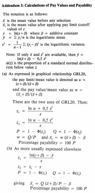
There have been two main approaches to these calculations. In 1962, Krige produced a graphical representation between the four quantities: pay limit/mean value, pay value/mean value, logarithmic variance, and percentage payability. The definition of any two of these quantities permits the direct calculation of the other two. This graph is in widespread use in the industry and can be regarded as definitive.
Other authors (e.g. David) have preferred to give the mathematical relationship and suggest that users calculate each result directly. In this approach, which is detailed in Addendum 3, the user must supply the parameters of the lognormal distribution and the pay limit to obtain the pay value and the payability. In addition to the mathematics, the user needs a table of the cumulative normal (Gaussian) distribution function. This is generally the first table in any set of statistical tables or textbook. To computerize this approach is the work of a moment, requiring only a routine for the normal function. Many algorithms are available for this function (e.g. Abramowitz and Stegun, p. 931). Algorithms such as 26.2.19 give up to seven significant figures in precision, in a range of six standard deviations on either side of the mean value.
One advantage of the graphical approach over the simple calculation is that the user can (say) define the desired pay value and read off the pay limit that must be applied to reach this goal. Similarly, the user can define payability and obtain the relevant pay limit and pay value. The latter can be carried out by a program simply by reversing the mathematics and using an algorithm for the inverse of the normal distribution function – such as the PPND discussed in the first section of this paper. It is much more difficult to calculate the results starting with a desired pay value, since the mathematics is complicated by two normal inverses. The usual answer to this, in practice, is to calculate the results for several pay limits and 'home in' on the desired pay value.
As far as timings are concerned, it is more efficient to use the (b) form of the mathematics given in Addendum 3. There is a very small overhead in the calculation of the logarithmic mean and in square-rooting the logarithmic variance. Apart from that, the timing costs should be constant per pay limit. On the Alpha Micro, single calculations of pay limits take around 0.03 seconds each. On any IBM PC (without coprocessor) the results appear on the screen with no perceptible pause. The entire GRL20 graph can be recreated in around 6 seconds on the Alpha Micro excluding the physical plotting time (which will depend on the plotter used).
The Additive Constant (Again)
The first section of this paper discussed the estimation of the third parameter – the additive constant. Krige states that the estimation of the mean value is robust with regard to the additive constant. We confirmed this empirically with a particular set of sample values. We also found that the lower confidence limit was stable, but that the logarithmic variance and the upper confidence limit were not. It would seem, then, that the choice of additive constant, within reasonable bounds, does not affect the final estimate of average value or of a lower confidence level on this estimate. Some concern has to be shown about the effect on the upper confidence limits but, since these are rarely used in practice, the problem is not of paramount importance.
However, we must accept that the estimate of the logarithmic variance changes considerably with the additive constant. As the constant rises, the logarithmic variance drops. In the calculation of pay limit/pay value/payability, the logarithmic variance is of great importance for there is not a single term in the calculation that does not depend on it. In the GRL20 graph there are separate lines for different variances. Perhaps it would be valuable to give an example of the effect of the choice of constant on the payability figures.
Table II gives the estimated average and logarithmic variance calculated according to Sichel's t procedure on the set of data in Table I and assuming various additive constants. The, variances change from over 1.4 with zero constant to 0.25 with a constant of 200. These sample values were simulated from a distribution with an additive constant of 100; at that level, the logarithmic variance is estimated at 0.426. We chose a set of pay limits between 300 and 1000 to apply to the distribution. The calculations were performed for additive constants of 0. 50, 100, 150, and 200, and the results are shown in Tables VII and VIII.
The first thing shown by the tables is that the assumption of no additive constant has a much greater effect than the assumption of an erroneous one. For example, at a pay limit of 300, there is a discrepancy of around 330 in the pay value and 9 per cent in the payability, as compared with the 'correct' value of 100 for the third parameter. This gap widens as the pay limits rise. Our first conclusion must be that, if the values are three parameter lognormal, some value must be used for the additive constant.
Closer inspection of Tables VII and VIII show that the percentage payability varies little with the additive constant. At most, the deviation from the 'expected' value is around 3 per cent, and this is for a low cutoff of 300. The more disturbing factor, perhaps, is that the mean value changes significantly. Taking additive constants ranging from one-half to twice the correct value, we find differences in the average value of 7 to 9 per cent.
It would seem, then, that the effort of finding a good estimate of the third parameter – the additive constant will be repaid with a significant increase in the precision of the payability calculations.
Conclusion
The aim in this paper was to illustrate the implementation of some of the traditional methods of reserve estimation on today's microcomputers. The main advantages of this type of computing power are the low costs both in purchase and in operating – and the ease of accessibility to those with a minimum of computer expertise. All of the illustrative examples and conclusions reached in this paper were produced on an in-house Alpha Micro at no extra cost to the company. This machine runs at about the same speed as an IBM PC AT without a coprocessor. With the coprocessor, the AT runs about 2.75 times faster (Williams et al). Obviously, timings are faster on minicomputers such as a Vax system. However, costs tend to rise also, since these machines are multi-user and tend to have well-developed accounting packages. The major point in favour of using a PC, then, is the very fact that it is designed to be 'personal' - single-user, low-cost, friendly system.
It has been shown that, for the most part, the techniques described in this paper present few problems in being converted to a computer form. Where decisions have to be made, e.g. on what approximations to accept, our approach has enabled us to evaluate many alternatives to make sure that the results really are optimum. We have found that the more traditional 'table and graph' approach can lead to some fairly major errors if not used with caution. We have also raised some questions that, we hope, will stimulate further consideration of some of the accepted approximations.
Finally, perhaps the author should reveal the real purpose in submitting this paper. Since the use of computers became widespread in the mineral industry, there has been a certain amount of pressure to take advantage of this by the use of more mathematical, more sophisticated, more complex, more costly, and more erudite techniques for the estimation of reserves. One has only to look at the development of Matheronian Geostatistics over the last twenty years for ample illustration of this process. Presented as a simple objective mathematical formulation of Krige's empirical work in the early 1960s by Matheron, it blossomed to fill textbooks by the late 1970s (e.g. David) and has since branched into at least three opposing schools of thought promoting their own variations of Ordinary Kriging, Simple Kriging, Disjunctive Kriging, Multivariate Gaussian Kriging, Probability Kriging, Indicator Kriging, and so on ad infinitum. All of these techniques, of course, are impossible without computers and very difficult without the appropriate software.
Although these methods are invaluable in their place, the more traditional proven methods have been overshadowed by the welter of theory, application, and controversy surrounding the newer techniques. It is time, perhaps, that the established methods be seen to resume their place as valuable weapons in the armoury of modern reserve estimation.
Acknowledgements
This work was carried out at the offices of Geostokos Limited in London, England. The author thanks the Geostatistics Department at Gencor in Johannesburg, particularly Dr C.T.P. Williams, for motivation and encouragement (and practical advice) in this study, and for assisting in the revision of the paper in the light of the referee's comments.
References
1. WAINSTEIN, B.M. An extension of lognormal theory and its application to risk analysis models for new mining ventures. J. S. Afr. Inst. Min. Metall., vol. 75. 1975. pp. 221-238.
2. SICHEL, H.S. New methods in the statistical evaluation of mine sampling data. Trans. Instn Min. Metall., vol. 61. 1952. pp. 261-288.
3. SICHEL, H.S. The estimation of means and associated confidence limits for small samples from lognormal populations. Symposium on Mathematical Statistics and Computer Applications in Ore Valuation. Johannesburg, The South African Institute of Mining and Metallurgy, 1966. pp. 106-122.
4. HALD, A. Statistical theory with engineering applications. London and New York, John Wiley & Sons, 1952. 783 pp.
5. KRIGE, D.G. A statistical approach to some mine valuation and allied problems on the Witwatersrand. M.Sc. (Eng.) thesis, University of the Witwatersrand, Johannesburg, 1951.
6. KRIGE, D.G. On the departure of ore value distributions from the lognormal model in South African gold mines. J. S. Afr. Inst. Min. Metall., vol. 61. 1960. pp. 231-244.
7. KRIGE, D.G. Lognormal-de Wijsian geostatistics for ore evaluation. Johannesburg, The South African Institute of Mining and Metallurgy, Monograph Series, Geostatistics 1, 1978. 50 pp.
8. RENDU, J-M. An introduction to geostatistical methods of mineral evaluation. Johannesburg, The South African Institute of Mining and Metallurgy, Monograph Series, Geostatistics 2, 1978. 84 pp.
9. BEASLEY, J. R., and SPRINGER, S. G. Algorithm AS 111. The percentage points of the normal distribution. Appl. Statist., vol. 26. 1977. pp. 118-121.
10. SICHEL, H.S. Development of large sample estimators for the 3-parameter lognormal distribution (Project 120/67). Manuscript, 1968. 33 pp.
11. CLARK, I., and GARNETT, R.H.T. Identification of multiple mineralisation phases by statistical methods. Trans. Instn Min. Metall., vol. 83. 1974. pp. 43-52.
12. CLARK, I. ROKE, A computer program for non-linear least squares decomposition of mixtures of distributions. Computers and Geosciences, vol. 3. 1977. pp. 245-256.
13. SICHEL, H.S. An experimental and theoretical investigation of bias error in mine sampling with special reference to narrow gold reefs. Trans. Instn Min. Metall., vol. 56. 1947. pp. 403-473.
14. DAVID, M. Geostatistical ore reserve estimation. Amsterdam, Elsevier, 1977. 364 pp.
15. ABRAMOWITZ, M., and STEGUN. I.A. Handbook of mathematical functions. New York, Dover Publications Inc., 1970. 104.6 pp.
16. KRIGE, D.G. Statistical applications in mine valuation. J. Inst. Min. Surv. S. Afr., vol. 12. 1962. pp. 45-84, 95-136.
17. WILLIAMS, C.T.P., CLARK, I., and SMITHIES, S.N. TRIPOD – A computer program for evaluating borehole sampling in gold projects. J. Inst. Min. Surv. S. Afr., vol. 23. 1986. pp. 109-116.
18. MATHERON, G. Principles of geostatistics. Economic Geology, vol. 58. 1963. pp. 1246-1266.
TABLES
TABLE I
A TEST SET OF DATA FOR THE INFLUENCE OF THE ADDITIVE CONSTANT ON VARIOUS PARAMETERS CALCULATED DURING A SICHEL'S t ANALYSIS
| 10.05 | 50.64 | 124.60 |
| 183.53 | 185.63 | 279.78 |
| 299.92 | 308.07 | 422.94 |
| 542.88 | 573.18 | 584.20 |
| 750.38 | 811.24 | 828.54 |
TABLE II
THE INFLUENCE OF THE ADDITIVE CONSTANT ON
SICHEL'S t ESTIMATOR AND OTHER PARAMETERS
| Additive | Estimated | Logarithmic | Lower | Upper |
| constant | average | variance | 95% Pt | 0.95% Pt |
| 0 | 500.7 | 1.422 | 300.5 | 1258.6 |
| 10 | 460.9 | 1.088 | 294.4 | 993.7 |
| 20 | 443.3 | 0.909 | 292.7 | 882.9 |
| 30 | 432.8 | 0.790 | 292.1 | 818.8 |
| 40 | 426.0 | 0.702 | 292.0 | 776.4 |
| 50 | 421.1 | 0.633 | 292.1 | 745.7 |
| 60 | 417.4 | 0.577 | 292.4 | 722.4 |
| 70 | 414.6 | 0.531 | 292.6 | 704.0 |
| 80 | 412.2 | 0.491 | 292.9 | 689.1 |
| 90 | 410.4 | 0.456 | 293.2 | 676.7 |
| 100 | 408.9 | 0.426 | 293.5 | 666.2 |
| 110 | 407.6 | 0.400 | 293.8 | 657.3 |
| 120 | 406.5 | 0.376 | 294.0 | 649.5 |
| 130 | 405.5 | 0.355 | 294.3 | 642.7 |
| 140 | 404.7 | 0.336 | 294.5 | 636.8 |
| 150 | 404.0 | 0.318 | 294.7 | 631.4 |
| 160 | 403.4 | 0.303 | 294.9 | 626.6 |
| 170 | 402.8 | 0.288 | 295.1 | 622.4 |
| 180 | 402.3 | 0.275 | 295.3 | 618.5 |
| 190 | 401.9 | 0.262 | 295.5 | 614.9 |
| 200 | 401.5 | 0.251 | 295.6 | 611.7 |
TABLE III
Ψ FACTORS FOR SICHEL'S t ESTIMATION FOR
10 SAMPLE VALUES AT 95% CONFIDENCE
| V | σ2 = 0.7 | σ2 = 0.3 | σ2 = 1.5 | σ2 = nV/(n-1) |
| 0.01 | 1.081 | 1.075 | 1.090 | 1.070 |
| 0.10 | 1.292 | 1.268 | 1.325 | 1.251 |
| 0.20 | 1.455 | 1.415 | 1.508 | 1.405 |
| 0.40 | 1.754 | 1.684 | 1.850 | 1.713 |
| 0.60 | 2.066 | 1.962 | 2.211 | 2.059 |
| 0.80 | 2.410 | 2.265 | 2.614 | 2.465 |
| 1.00 | 2.798 | 2.604 | 3.074 | 2.951 |
| 1.50 | 4.033 | 3.667 | 4.565 | 4.658 |
| 2.00 | 5.803 | 5.163 | 6.760 | 7.453 |
TABLE IV
TIMING IN SECONDS FOR SINGLE CONFIDENCE LEVELS CALCULATED FOR VARIOUS VALUES OF n AND p
| Number of | Log variance | Percentage points | ||
| samples | σ2 | p=2.5% | p=5% | p= 10% |
| 5 | 0.3 | 61 | ||
| 5 | 0.7 | 93 | 122 | 137 |
| 5 | 1.5 | 138 | 177 | 225 |
| 10 | 0.3 | 71 | ||
| 10 | 0.7 | 126 | 131 | 157 |
| 10 | 1.5 | 201 | 209 | 272 |
| 15 | 0.3 | 63 | ||
| 15 | 0.7 | 119 | 136 | 134 |
| 15 | 1.5 | 211 | 221 | 239 |
| 20 | 0.3 | 62 | ||
| 20 | 0.7 | 128 | 142 | 145 |
| 20 | 1.5 | 240 | 242 | 242 |
TABLE V Ψ FACTORS FOR SICHEL'S t ESTIMATION FOR 10 SAMPLE VALUES ASSUMING σ2 = 0.7
| Percentage points | ||||||||||
| V | γn(V) | 1 | 2.5 | 5 | 10 | 50 | 90 | 95 | 97.5 | 99 |
| 0.01 | 1.0050 | 0.933 | 0.944 | 0.952 | 0.962 | 1.001 | 1.059 | 1.081 | 1.104 | 1.135 |
| 0.02 | 1.0100 | 0.907 | 0.921 | 0.933 | 0.947 | 1.002 | 1.085 | 1.117 | 1.151 | 1.197 |
| 0.04 | 1.0202 | 0.871 | 0.890 | 0.907 | 0.926 | 1.003 | 1.123 | 1.172 | 1.222 | 1.292 |
| 0.06 | 1.0304 | 0.844 | 0.868 | 0.887 | 0.910 | 1.005 | 1.154 | 1.216 | 1.280 | 1.371 |
| 0.08 | 1.0407 | 0.822 | 0.849 | 0.871 | 0.897 | 1.006 | 1.182 | 1.256 | 1.333 | 1.444 |
| 0.10 | 1.0510 | 0.803 | 0.832 | 0.856 | 0.885 | 1.007 | 1.208 | 1.292 | 1.382 | 1.511 |
| 0.12 | 1.0615 | 0.786 | 0.817 | 0.844 | 0.875 | 1.009 | 1.231 | 1.327 | 1.428 | 1.577 |
| 0.14 | 1.0720 | 0.771 | 0.804 | 0.832 | 0.866 | 1.010 | 1.254 | 1.360 | 1.473 | 1.64 |
| 0.16 | 1.0826 | 0.756 | 0.792 | 0.821 | 0.857 | 1.012 | 1.276 | 1.392 | 1.517 | 1.702 |
| 0.18 | 1.0934 | 0.743 | 0.780 | 0.811 | 0.849 | 1.013 | 1.298 | 1.424 | 1.560 | 1.764 |
| 0.20 | 1.1042 | 0.731 | 0.769 | 0.802 | 0.841 | 1.015 | 1.319 | 1.455 | 1.603 | 1.825 |
| 0.30 | 1.1595 | 0.678 | 0.723 | 0.762 | 0.809 | 1.022 | 1.420 | 1.605 | 1.812 | 2.132 |
| 0.40 | 1.2171 | 0.635 | 0.685 | 0.728 | 0.781 | 1.030 | 1.518 | 1.754 | 2.025 | 2.453 |
| 0.50 | 1.2770 | 0.598 | 0.652 | 0.699 | 0.758 | 1.039 | 1.617 | 1.907 | 2.246 | 2.796 |
| 0.60 | 1.3394 | 0.565 | 0.623 | 0.674 | 0.737 | 1.049 | 1.718 | 2.066 | 2.480 | 3.168 |
| 0.70 | 1.4044 | 0.537 | 0.597 | 0.651 | 0.718 | 1.059 | 1.823 | 2.234 | 2.731 | 3.574 |
| 0.80 | 1.4719 | 0.510 | 0.573 | 0.630 | 0.701 | 1.070 | 1.932 | 2.410 | 3.000 | 4.021 |
| 0.90 | 1.5420 | 0.486 | 0.551 | 0.610 | 0.685 | 1.081 | 2.047 | 2.598 | 3.290 | 4.514 |
| 1.00 | 1.6150 | 0.464 | 0.531 | 0.592 | 0.671 | 1.093 | 2.167 | 2.798 | 3.604 | 5.058 |
| 1.10 | 1.6908 | 0.444 | 0.512 | 0.575 | 0.657 | 1.106 | 2.294 | 3.012 | 3.945 | 5.662 |
| 1.20 | 1.7695 | 0.425 | 0.495 | 0.560 | 0.644 | 1.120 | 2.427 | 3.241 | 4.315 | 6.331 |
| 1.30 | 1.8515 | 0.408 | 0.478 | 0.545 | 0.633 | 1.134 | 2.569 | 3.486 | 4.717 | 7.073 |
| 1.40 | 1.9365 | 0.391 | 0.463 | 0.531 | 0.621 | 1.149 | 2.718 | 3.750 | 5.155 | 7.898 |
| 1.50 | 2.0248 | 0.376 | 0.449 | 0.518 | 0.611 | 1.165 | 2.877 | 4.033 | 5.633 | 8.815 |
| 1.60 | 2.1164 | 0.362 | 0.435 | 0.506 | 0.601 | 1.182 | 3.045 | 4.337 | 6.154 | 9.834 |
| 1.70 | 2.2116 | 0.348 | 0.423 | 0.495 | 0.592 | 1.200 | 3.224 | 4.664 | 6.722 | 10.968 |
| 1.80 | 2.3194 | 0.336 | 0.411 | 0.484 | 0.584 | 1.218 | 3.413 | 5.016 | 7.341 | 12.231 |
| 1.90 | 2.4128 | 0.324 | 0.399 | 0.474 | 0.576 | 1.238 | 3.615 | 5.395 | 8.018 | 13.636 |
| 2.00 | 2.5192 | 0.313 | 0.389 | 0.464 | 0.568 | 1.258 | 3.829 | 5.803 | 8.758 | 15.200 |
TABLE VI
Ψ FACTORS FOR SICHEL'S t ESTIMATION FOR
UPPER 95% CONFIDENCE ASSUMING σ2 = 0,7
| n=8 | Difference | ||||
| V | n=5 | n=10 | n=8 | Interpolated | % |
| 0.01 | 1.165 | 1.081 | 1.099 | 1.115 | 1.43 |
| 0.02 | 1.243 | 1.117 | 1.144 | 1.167 | 2.08 |
| 0.04 | 1.364 | 1.172 | 1.211 | 1.248 | 3.07 |
| 0.0445 | 1.388 | 1.182 | 1.225 | 1.265 | 3.26 |
| 0.06 | 1.467 | 1.216 | 1.267 | 1.316 | 3.89 |
| 0.10 | 1.653 | 1.292 | 1.364 | 1.437 | 5.32 |
| 0.20 | 2.088 | 1.455 | 1.575 | 1.708 | 8.46 |
| 0.50 | 3.568 | 1.907 | 2.189 | 2.571 | 17.48 |
| 1.00 | 7.618 | 2.798 | 3.491 | 4.726 | 35.40 |
| 1.50 | 15.601 | 4.033 | 5.446 | 8.660 | 59.03 |
| 2.00 | 31.473 | 5.803 | 8.472 | 16.071 | 89.69 |
| 3.00 | 124.149 | 12.142 | 20.641 | 56.945 | 175.88 |
TABLE VII
COMPARISON OF PAY VALUES WHEN
DIFFERENT ADDITIVE CONSTANTS ARE ASSUMED
| Additive constant | |||||||
| Pay limit | 0 | 50 | 90 | 100 | 110 | 150 | 200 |
| 300 | 978 | 699 | 652 | 645 | 639 | 619 | 605 |
| 400 | 1148 | 818 | 759 | 749 | 741 | 716 | 697 |
| 500 | 1316 | 938 | 869 | 858 | 848 | 818 | 794 |
| 600 | 1480 | 1059 | 981 | 968 | 957 | 922 | 894 |
| 700 | 1642 | 1181 | 1094 | 1079 | 1067 | 1028 | 996 |
| 800 | 1802 | 1303 | 1207 | 1192 | 1178 | 1135 | 1100 |
| 900 | 1961 | 1425 | 1322 | 1304 | 1290 | 1243 | 1204 |
| 1000 | 2118 | 1547 | 1436 | 1417 | 1401 | 1351 | 1310 |
TABLE VIII
COMPARISON OF PAYABILITY VALUES WHEN
DIFFERENT ADDITIVE CONSTANTS ARE ASSUMED
| Additive constant | |||||||
| Pay limit | 0 | 50 | 90 | 100 | 110 | 150 | 200 |
| 300 | 43 | 49 | 51 | 52 | 52 | 53 | 55 |
| 400 | 34 | 37 | 38 | 38 | 38 | 39 | 40 |
| 500 | 28 | 28 | 28 | 28 | 28 | 29 | 29 |
| 600 | 23 | 21 | 21 | 21 | 21 | 21 | 21 |
| 700 | 19 | 16 | 16 | 15 | 15 | 15 | 15 |
| 800 | 16 | 13 | 12 | 11 | 11 | 11 | 10 |
| 900 | 14 | 10 | 9 | 9 | 8 | 8 | 7 |
| 1000 | 11 | 8 | 7 | 7 | 6 | 6 | 5 |
ADDENDA