ABSTRACT

Most statistical and geostatistical methods of resource and reserve estimation work extremely well for Normal (Gaussian) well-behaved information. However, most interesting mineral deposits exhibit far from this idealistic distribution of values. It seems that the more valuable the mineral, the less likely the data are to have a Normal distribution. Values tend to be "positively skewed" with a long tail into the high values. Using averaging techniques, such as inverse distance or ordinary kriging may result in considerable overestimation of grades and tonnages unless such values are cut or otherwise modified.

This paper presents some real case studies where distributions are (a) highly skewed and (b) the product of multiple phases of mineralisation. Practical methods are presented for solving such problems – including combinations of indicator and lognormal kriging methods. The emphasis of the presentation is on developing operational methods which can be used on project evaluation or grade control in producing mines.

INTRODUCTION

In the last twenty years of practical reserve and resource estimation several obvious trends have been observed:

Computers

  Ø   The increase of availability of computing power – particularly of personal computers and workstations – has encouraged the computerisation of the large majority of mining ventures world-wide. It is common now for geological information to be computerised as exploration proceeds although, in many parts of the world, long established producing mines are still going through the mild trauma of upgrading sampling and surveying data to computers.

  Ø   The availability of computers and of specialised software has encouraged the use of more complex methods of resource estimation. Of these, perhaps the most spectacular rise has been that of the geostatistical methods. The potential of geostatistical methods to produce the 'optimal' estimator and to provide confidence levels on those estimations is a powerful motive to change from simpler, less objective approaches.

Economics

Mineral deposits being discovered and brought into production have become more marginal economically in recent years. In addition, more pressure is being brought to bear by potential investors – whether banks, parent companies or individuals – to quantify the confidence in or reliability of stated reserves. Committees have been set up in many countries to specify acceptable definitions for "proven" or "measured" resources and reserves.

As economic cutoffs rise in parallel with mining costs and accessibility, the "shape" of the mineral distribution becomes more important. Rising cutoffs have far more impact on skewed distributions than on comparatively "Normal" ones. The further into the 'tail' of the values, the more biassed most resource estimation methods become. Weighted average type estimators such as inverse distance and kriging are unbiassed over the whole deposit, but conditionally biassed once cutoffs are applied. These estimators are also biassed for skewed distributions – the more skewed, the more biassed. Questions arise as to whether high values should be cut to provide more "conservative" estimates or whether more sophisticated techniques need to be applied.

Geology

As the richer and more obvious deposits are worked out, exploration produces more marginal and more geologically complex deposits for consideration. Geological controls such as faulting, folding and intrusions can now be modelled by computer and taken into account automatically when allocating values to potential mining blocks.

Less easy to control or, sometimes, identify are problems associated with mixtures of mineralisations. Mineral types can often be logged with host rock type when examining core. Obvious differences such as oxidation zones can be separated out as distinct geological units. Mineralisation phases, such as reworking or remobilisation, can often be identified by associated minerals or other visual characteristics. However, there are cases where complex deposition either cannot be visually assessed in the samples or is not identified when logging the core.

If any combination of these factors is ignored in the reserve valuation process, erroneous results can be obtained. No matter how sophisticated your software or how complex your geostatistical evaluation methods, ignoring the true complexity of the geology will produce the wrong answers.

This paper discusses how some of these factors may be included in resource and reserve estimation without the need to resort to highly complex mathematical processes and/or vastly increased amounts of data analysis. All of the cases presented in this paper are real projects or producing mines. Some of them are new projects and some are well-established mining ventures.

CASE STUDY

For simplicity we will use a small set of data to illustrate what can go wrong if complexities are not identified. The scale of the sample measurements is, in this context, arbitrary and fairly irrelevant to the issues under discussion. A post plot of the sample data, shaded by value is shown below. The samples average 275 units with a calculated standard deviation of 841.

Figure 1. Post plot of sample values and lease area

To get a rough idea of how the values vary, we can produce an inverse distance map for the lease area. It is obvious, from inspection, that values are more continuous 'along' the area than 'across' it. The search radius along the main axis of sampling was taken as twice that across the area. Radii were chosen to give approximately 16-20 samples for each estimation. An inverse distance squared technique was selected as this closely approximates ordinary kriging if the search ellipse is chosen correctly.

Figure 2 shows the map obtained from inverse distance estimation. It is fairly obvious that the few very high values have smeared themselves out along the search ellipse, giving the impression of a cohesive 'payable' central area. The estimated points average 282 units with a standard deviation of 288. An average of 24 samples was used in estimating each grid point.

Apart from some obvious smoothing, there doesn't seem to be much problem with 'bias'. Now, let us apply an arbitrary cutoff of 100 units. Of around 150 samples, just under 30% of the samples lie above 100 units. These average over 900 units with a standard deviation of 1400. Of the estimated points, just over 55% have values over 100 units. These have a average of 475 units with a standard deviation of 255.

The first question that comes to mind is, "have we chosen the correct search radius?". The simplest way to answer this question is to construct semi-variogram graphs. A semi-variogram is a graph of the 'relationship' between sample values versus the distance between them. If an 'inverse distance' type of relationship exists, this graph should tell us what it looks like.

The different symbols indicate the direction in which the graph was constructed. Since we are fairly sure there should be a difference with direction, we take pairs of samples in each direction and find out how different they are. According to this graph there is no pattern no matter what direction we look in. This suggests (in the absence of any other factors) that there is no relationship with distance and that, therefore, we should not be using a distance weighting technique at all. This conclusion does not seem sensible when we can see from the post plot that there is a distinct pattern in the sample values which should be reflected by this graph.

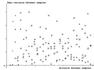
Figure 3. Semi-variograms calculated on sample values

STATISTICAL ANALYSIS

Since there is visual continuity in the sample values but none in the semi-variogram graph, it would seem that we have done something wrong with our analysis. The semi-variogram graph is calculated by finding pairs of samples a specified distance apart and in a specified direction. The difference in value is calculate for each pair. This is squared and averaged. For a semi-variogram one-half of this 'variance' is plotted against the distance between the samples. This works extremely well for Normal (Gaussian) type data where the variance of values is a sensible measure of variation. It does not work too well with skewed data. The graph below shows the histogram of the sample data values.

Figure 4. Histogram of sample values

This is highly skewed, as was indicated by the fact that the standard deviation is three times the mean value. Superimposing a lognormal distribution on this histogram gives an acceptable fit. This suggests that if we take logarithms of the values, we will have a Normal distribution. This should solve the problem of getting a valid semi-variogram graph. The graph in Figure 5 was calculated on the logarithm of the sample values. The same directions were used as before.

To be able to use kriging, we fit models to each.

If we accept the lognormal method, we have two options according to generally accepted practice. We could use the full lognormal kriging (and assume that the samples are actually lognormal) or we can use the "lognormal shortcut". In the latter case, we use the logarithmic semi-variogram models but we krige using the actual untransformed sample values. The two maps below show the difference between accepting the lognormal model and trying the shortcut approximation.

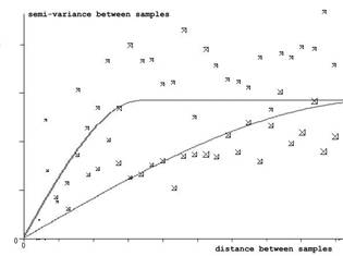
Figure 5. Semi-variograms calculated and modelled on logarithm of sample value

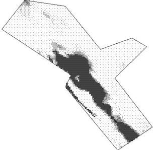
Figure 6: Kriging with raw sample values and logarithmic semi-variogram model

Figure 7. Full lognormal kriging with backtransformation

The lognormal shortcut produces a grid which averages 196 units with standard deviation 493. The full lognormal kriging averages 157 with a standard deviation of 379. Neither of these is anywhere near the characteristics of the original sample data. Applying a cutoff of 100 units gives 30% payable at an average of 618 for lognormal shortcut and 27% payable at an average of 518 units for the full lognormal approach.

Whilst these two maps are giving something closer to what we expect from the sample data, neither of them are very satisfactory in terms of recoverable grades. The lognormal shortcut shows instability – check out that strange high value area in the south-west. The lognormal approach is giving a sensible map in that it reflects the original visual assessment of the data. However, the "recoverable reserves" are disappointing.

We do not expect to obtain the average and standard deviation witnessed in the original sample values, but it would certainly be reassuring to get something close enough to give us confidence that our geostatistical model is actually representing the geology of the deposit.

MORE COMPLEX APPROACHES

Going back to a visual assessment of the sample data, it would appear that there is a central area which is 'payable' surrounded on all sides by unpay ground. None of the approaches described above incorporate that image in any way. It would seem sensible to find a model which looks like our concept of the deposit.

Since there is a cohesive central (generally) high grade area, this suggests that a kriging method including a 'drift' or trend in values might be what is needed. The simplest way to do this is to use 'universal' kriging which adds a simple polynomial type trend to the kriging equations.

We tried that in this case and obtained the map shown in Figure 8.

Figure 8: lognormal kriging with polynomial trend

Since fitting a trend also demands Normal type data, this is a variant on the lognormal kriging used above to produce Figure 7. Essentially, Figure 8 is just Figure 7 with the instruction to keep going in a certain direction if there is a strong trend in the data. For example, the values fall off rapidly from the central high value area. This is extended by including the trend in the kriging calculation.

The points on this map average 235 units with a standard deviation of 666. Since the trend component makes sure that the values drop off all round the edges, this is a pretty good match to the data. At a cutoff of 100 units, around 26% of the area is payable at an average of 680 units. The standard deviation on these values is around 1050 (compare to sample values at 1400).

Alternatives

In this case the deposit is a cohesive central core with values dropping off in all directions. This is a perfect case for kriging with a polynomial type trend. In other cases, the 'pay' and 'unpay' areas are too intermingled to be separated in this way. Another diagnostic for the need to apply a more complex method is simply to look at a probability plot of the data rather than a histogram. In this case, the probability plot shows a clear deviation from standard lognormality. We could have picked up the need for distinguishing the two subregions sooner if we had looked at this graph earlier.

Figure 9. Probability plot of sample values

The 'kink' (point of inflexion) clearly visible in this plot is diagnostic of the existence of two geological factors in the sample values. In 25 years of inspecting such graphs, we have found that every such kink has had a recognisable geological reason. In this simple illustration, the mixture is simply pay/ unpay. In fact, the kink occurs at a relative value of 45, not 100. This implies that the geological discrimination takes place at 45 units rather than the economic cutoff of 100 units.

It is always better to model the geology of a deposit and leave economics until the last stage of evaluation.

Base Metal example

In other cases, the delineation between two (or three) mineralisations is not so clear. In a recent base metal project in Namibia, three hydrothermal events were present throughout the deposit. Taking volumes as small as 200 by 200 by 20 metres did not produce simplified histograms. At all scales, three components were recognisable. The histogram of values is shown in Figure 10 below.

Figure 10. Histogram of logarithms of sample values

The three phases could not be identified in the borehole cores and could not be delineated in the computer geological model. Trends in values did not produce acceptable models. In this case it was necessary to combine different methods of kriging in order to produce a reliable block by block reserve estimate for mine planning purposes.

It proved impossible, by statistical methods, to separate the upper two components of the distribution. An indicator kriging was used for each block to identify how much of the block was likely to be in the low grade 'background' component. The remainder was assumed to be composed of payable medium and high grade material. The grade for this material was evaluated using a lognormal kriging approach.

In this way, a practical and reliable reserve estimation method was produced by combining two established techniques – one indicator kriging and one lognormal kriging run. Validations were run and visual comparison with borehole sections carried out to verify the results.

Precious metal example

Gold and platinum deposits are often composed of multiple phases of mineralisation, of massive reworking and remobilisation, or of major oxidation zones. In many cases, combinations of indicator and lognormal methods can be effective in improving resource estimation and obtaining more realistic figures.

There are some case, though, which can be handled with a simpler approach. The probability plot in Figure 11 looks like an ideal straight line fit. The values plotted in this figure are, however, the logarithm of the sample values after a constant value has been added to each. This model is known as the "three parameter lognormal" and can be used in many cases where a simple lognormal plot produces heavily biassed figures.

Figure 11. Probability plot of gold values using a three parameter lognormal model.

SUMMARY

The intent of this paper is to try to illustrate the improvement in resource and reserve estimation which can be achieved by reasonably simple geostatistical methods combined with a thorough understanding of the geological structure of the deposit under valuation.

All too often the failure to adequately value a project or control grades within a producing mine is blamed on the computer software or techniques being applied. It is in the selection of the appropriate technique that the expertise of a good ore reserve analyst lies. Good resource estimation is a synthesis of geological knowledge, computer expertise and statistical techniques. It is, in short, only achievable by a team effort.